前言 在上一篇文章[机器学习基础笔记(一)] 中,笔者整理了机器学习这门课上半节的课程内容,由于博客目录存在容量上限,之后的内容目录会无法显示,因此为了美观起见,在此重开一篇文章,作为该系列的第二部分
当然,目前课程还未结束,本文会随着课程进度,同步更新。
由于当前内容已经超出本文目录结构所能承载的极限,故本文完结,后续内容将在[机器学习基础笔记(三)] 中继续。
树,森林,与集成学习(Trees, Forests & Ensembles) 这个标题看着竟然有些文艺。
树模型(Tree Models) 简介是网上复制来的:
决策树(Decision Tree)是树模型中最简单的一个模型,也是后面将要介绍到的随机深林与梯度提升决策树两个模型的基础。利用决策树算法,在历史数据集上,我们可以画出这样一个树,这颗树上的叶子节点表示结论,非叶子节点表示依据。一个样本根据自身特征,从根节点开始,根据不同依据决策,拆分成子节点,直到只包含一种类别(即一种结论)的叶子节点为止。
代码:
1
2
3
4
from sklearn.tree import DecisionTreeRegressortree = DecisionTreeRegressor() tree.fit(X_train, y_train)
可以用这个代码可视化:
1
2
3
4
5
from sklearn.tree import plot_tree%matplotlib inline fig = plt.figure(figsize=(25 ,20 )) _ = plot_tree(tree, filled=True )
特征重要性:
1 plt.barh(cols, tree.feature_importances_)
当然,单一树模型不调参会有过拟合问题,因此进行网格搜索调参:
1
2
3
4
5
6
7
8
9
10
11
12
13
14
15
16
17
18
19
20
21
22
regtree = DecisionTreeRegressor() parameters={"splitter" :["best" ,"random" ], "max_depth" : [1 ,3 ,5 ], "min_samples_leaf" :[1 ,2 ,3 ,4 ,5 ], "min_weight_fraction_leaf" :[0.1 ,0.2 ,0.3 ], "max_features" :["auto" ,"log2" ,"sqrt" ,None ], "max_leaf_nodes" :[None ,10 ,20 ] } from sklearn.model_selection import GridSearchCVfrom sklearn.metrics import mean_squared_error, make_scorermy_mse = make_scorer(mean_squared_error, greater_is_better=False ) tuning_model = GridSearchCV(regtree, param_grid=parameters, scoring=my_mse, cv=3 ,) tuning_model.fit(X_train, y_train) tuning_model.best_params_
得到:
1 2 3 4 5 6 {'max_depth' : 5 , 'max_features' : 'log2' , 'max_leaf_nodes' : 20 , 'min_samples_leaf' : 4 , 'min_weight_fraction_leaf' : 0.1 , 'splitter' : 'best' }
集成学习(Ensemble Learning) 定义是网上复制来的:
集成学习(Ensemble Learning)算法的基本思想就是将多个分类器组合,从而实现一个预测效果更好的集成分类器。
随机森林模型(Random Forests) 定义是网上复制来的:
随机森林,顾名思义,是用随机的方式建立一个森林,森林里面有很多的树模型,随机森林的每一棵树之间是没有关联的。 在得到森林之后,当有一个新的输入样本进入的时候,就让森林中的每一棵树分别进行一下判断,看看这个样本应该属于哪一类(对于分类算法),然后看看哪一类被选择最多,就预测这个样本为那一类。
代码:
1
2
3
4
from sklearn.ensemble import RandomForestRegressorfor1 = RandomForestRegressor() for1_fit = for1.fit(X_train, y_train)
特征重要性:
1 plt.barh(cols, for1.feature_importances_)
调参:
1
2
3
4
5
6
7
8
9
10
11
12
13
14
15
16
17
18
19
20
21
22
23
24
rantree = RandomForestRegressor() parameters={'bootstrap' : [True ], 'max_depth' : [80 , 90 , 100 ], 'max_features' : ['auto' , 'sqrt' ], 'min_samples_leaf' : [2 , 3 ], 'min_samples_split' : [3 , 4 , 5 ], 'n_estimators' : [200 , 400 ]} from sklearn.model_selection import GridSearchCVfrom sklearn.metrics import mean_squared_error, make_scorermy_mse = make_scorer(mean_squared_error, greater_is_better=False ) tuning_model = GridSearchCV(rantree, param_grid=parameters, scoring=my_mse, cv=3 , n_jobs = -1 , verbose = 2 ) tuning_model.fit(X_train, y_train) tuning_model.best_params_
得到:
1 2 3 4 5 6 {'bootstrap' : True , 'max_depth' : 80 , 'max_features' : 'sqrt' , 'min_samples_leaf' : 2 , 'min_samples_split' : 3 , 'n_estimators' : 200 }
梯度上升模型(Gradient Boosting Trees) 不介绍定义以及数学原理了,需要的时候搜索一下就行,主要记录下一些代码实现。
1
2
3
4
from sklearn.ensemble import GradientBoostingRegressorfor2 = GradientBoostingRegressor() for2_fit = for2.fit(X_train, y_train)
特征重要性:
1 plt.barh(cols, for2.feature_importances_)
调参:
1
2
3
4
5
6
7
8
9
10
11
12
13
14
15
16
17
18
19
20
21
22
gratree = GradientBoostingRegressor() parameters={'max_depth' : [80 , 90 , 100 ], 'max_features' : ['auto' , 'sqrt' ], 'min_samples_leaf' : [2 , 3 ], 'min_samples_split' : [3 , 4 , 5 ], 'n_estimators' : [200 , 400 ]} from sklearn.model_selection import GridSearchCVfrom sklearn.metrics import mean_squared_error, make_scorermy_mse = make_scorer(mean_squared_error, greater_is_better=False ) tuning_model2 = GridSearchCV(gratree, param_grid=parameters, scoring=my_mse, cv=3 , n_jobs = -1 , verbose = 2 ) tuning_model2_fit = tuning_model2.fit(X_train, y_train) tuning_model2_fit.best_params_
究极梯度上升(XGBoost) 其实这个中文翻译大家都是叫极限梯度上升的,但本人图一乐,觉得“究极”这词看起来有趣一些,就在本文里这么叫了,大佬轻喷。
这部分不仔细写了,和上述三个是大同小异的。
线性分类模型(Linear Models for Classification) 逻辑回归(Logistic Regression) 逻辑回归,是用来做分类的一种线性模型。由于本学渣的数学知识储备不足以理解明白这模型的底层实现原理,这里就不多写了。
1
2
3
4
5
6
7
8
from sklearn.pipeline import Pipelinefrom sklearn.linear_model import LogisticRegressionfrom sklearn.preprocessing import RobustScalersteps = [('Rescale' , RobustScaler()), ('lr' , LogisticRegression())] model = Pipeline(steps)
支持向量机(Support Vactor Machine) 支持向量机,简称SVM,是一种分类器算法。
具体数学原理超出本人能力,就不在这里描述了。
边界(Margin) 当数据集可以严格二分时,设置硬边界(Hard Margin),否则设置软边界(Soft Margin)。
核函数(Kernel ) 当数据不可线性分割时,通过设置核函数(Kernel Fuction)升维,然后在高维数据中获取超平面(HyperPlane),再将超平面降维得到边界函数。
用于升维的核函数有很多,如RBF核、多项式核、Sigmoid核等等。一般RBF可以作为一切数据的核函数,当然容易会有过拟合问题。
要调的参数为C和gamma,调节前需要对数据放缩。
网格搜索调参:
1
2
3
4
5
param_grid = {'svc__C' : np.logspace(-3 , 2 , 6 ), 'svc__gamma' : np.logspace(-3 , 2 , 6 ) / X_train.shape[1 ]} grid = GridSearchCV(scaled_svc, param_grid=param_grid, cv=10 ) grid.fit(X_train, y_train)
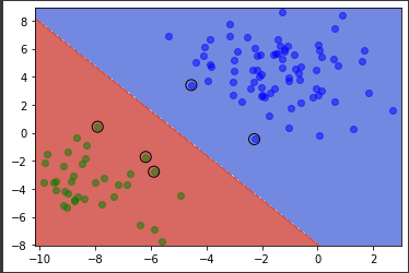
搭建一个简单的Pipeline并对支持向量可视化:
1
2
3
4
5
6
7
8
9
10
11
12
13
14
15
16
17
18
19
20
21
22
23
24
25
26
27
28
29
30
31
32
33
34
35
36
37
38
39
40
41
42
43
44
from sklearn.svm import SVCfrom sklearn.preprocessing import StandardScalerfrom sklearn.pipeline import make_pipelinefrom sklearn.pipeline import Pipelinescaler = StandardScaler() model = Pipeline([('scaler' , scaler), ('svc' , SVC(kernel='linear' ))]) model.fit(X.values, y) import numpy as npimport matplotlib.pyplot as plt%matplotlib inline x_min, x_max = df.iloc[:, 0 ].min () - 0.3 , df.iloc[:, 0 ].max () + 0.3 y_min, y_max = df.iloc[:, 1 ].min () - 0.3 , df.iloc[:, 1 ].max () + 0.3 xx, yy = np.meshgrid(np.arange(x_min, x_max, 0.02 ), np.arange(y_min, y_max, 0.02 )) Z = model.predict(np.c_[xx.ravel(), yy.ravel()]) Z = Z.reshape(xx.shape) plt.contourf(xx, yy, Z, cmap=plt.cm.coolwarm, alpha=0.8 ) plt.scatter(df[df.label == 0 ].x, df[df.label == 0 ].y, marker = 'o' , color = 'blue' , alpha = 0.5 , label = 'label = 0' ) plt.scatter(df[df.label == 1 ].x, df[df.label == 1 ].y, marker = 'o' , color = 'green' , alpha = 0.5 , label = 'label = 1' ) support_vectors = scaler.inverse_transform(model[1 ].support_vectors_) plt.scatter( support_vectors[:, 0 ], support_vectors[:, 1 ], s=100 , linewidth=1 , facecolors="none" , edgecolors="k" , )
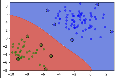
为支持向量机加核函数:
1
2
3
4
5
6
7
8
9
10
11
12
13
14
15
16
17
18
19
20
21
22
23
24
25
26
27
28
29
30
31
32
33
34
35
36
37
38
model = Pipeline([('scaler' , scaler), ('svc' , SVC(gamma='auto' , kernel='rbf' , C=1 , class_weight='balanced' ))]) model.fit(X.values, y) import numpy as npimport matplotlib.pyplot as plt%matplotlib inline x_min, x_max = df.iloc[:, 0 ].min () - 0.3 , df.iloc[:, 0 ].max () + 0.3 y_min, y_max = df.iloc[:, 1 ].min () - 0.3 , df.iloc[:, 1 ].max () + 0.3 xx, yy = np.meshgrid(np.arange(x_min, x_max, 0.02 ), np.arange(y_min, y_max, 0.02 )) Z = model.predict(np.c_[xx.ravel(), yy.ravel()]) Z = Z.reshape(xx.shape) plt.contourf(xx, yy, Z, cmap=plt.cm.coolwarm, alpha=0.8 ) plt.scatter(df[df.label == 0 ].x, df[df.label == 0 ].y, marker = 'o' , color = 'blue' , alpha = 0.5 , label = 'label = 0' ) plt.scatter(df[df.label == 1 ].x, df[df.label == 1 ].y, marker = 'o' , color = 'green' , alpha = 0.5 , label = 'label = 1' ) support_vectors = scaler.inverse_transform(model[1 ].support_vectors_) plt.scatter( support_vectors[:, 0 ], support_vectors[:, 1 ], s=100 , linewidth=1 , facecolors="none" , edgecolors="k" , )
模型评估(Model evaluation) 当我们基于各种算法,得到了一个分类器后,我们自然地就想知道,手头的这个分类器的性能如何。然而,什么是“性能好”,什么是“性能坏”呢?这里的量度该如何确定呢?
可能直觉上,我们会将测试数据输入模型,得到预测结果,用预测结果与实际数据对比,如果预测的正确率越高,同时错误率越低,则我们认为模型越好。
然而,用这样的量度训练模型,则会出现一些问题,如:
例1:恐怖分子识别任务。这是一个二分问题,恐怖分子计为正,非恐怖分子记为负。
这个任务的特点是:正例负例分布非常不平均,因为恐怖分子的数量远远小于非恐怖分子的数量。假设一个数据集内的恐怖分子与非恐怖分子数量比例为1:999999999,此时我们引入一个二分类判别模型,它的行为是将所有样例都识别为负例(非恐怖分子),那么在这个数据集上该模型的准确率高达99.9999999%(因为大部分都不是恐怖分子),但恐怕没有任何一家航空公司会为这个模型买单,因为它永远不会识别出恐怖分子,航空公司更关注有多少恐怖分子被识别了出来。
现实中这样的例子还有很多,在一背景下,我们需要一些新量度,来多方位的评判模型。
混淆矩阵(Confusion Matrix) 混淆矩阵是将一些模型评估量度可视化的一种方法,其记录真阳性(True Positive)、假阳性(False Positive)、真阴性(True Negative)、假阴性(True Negative)四个数据,这几个量度内容如下图,很生动了,本人就不再赘述。
将混淆矩阵中的量度进行一些计算,则可以得到新的指标:
精确率(Precision):
$Precision = \frac{TP}{TP+FP}$
Precision描述了正例结果中有多少是真实正例,即该二分类器预测的正例有多少是准确的
召回率(Recall)
$Recall = \frac{TP}{TP+FN}$
Recall描述了模型找到正例的能力
F值(F-Score)
$F = \frac{2Precision*Recall}{Precision + Recall}$
通过更改阈值(Threshold)可以得到不同的结果:
1
2
3
4
5
6
data = load_breast_cancer() X_train, X_test, y_train, y_test = train_test_split( data.data, data.target, stratify=data.target, random_state=0 ) lr = LogisticRegression().fit(X_train, y_train) y_pred = lr.predict(X_test) print (classification_report(y_test, y_pred))
precision
recall
f1-score
support
0
0.91
0.92
0.92
53
1
0.96
0.94
0.95
90
avg/total
0.94
0.94
0.94
143
1
2
y_pred = lr.predict_proba(X_test)[:, 1 ] > .85 print (classification_report(y_test, y_pred))
precision
recall
f1-score
support
0
0.84
1.00
0.91
53
1
1.00
0.89
0.94
90
avg/total
0.94
0.93
0.93
143
精度召回曲线(Precision-Recall Curve) 可以看到,当阈值变化时,上述指标都会变化,且Precision和Recall呈负相关,那么这两个指标的综合性能该如何体现?这时我们可以绘制Precision-Recall曲线(简称PRC)图:
1
2
3
4
5
6
X, y = make_blobs(n_samples=(2500 , 500 ), cluster_std=[7.0 , 2 ], random_state=22 ) X_train, X_test, y_train, y_test = train_test_split(X, y) svc = SVC(gamma=.05 ).fit(X_train, y_train) precision, recall, thresholds = precision_recall_curve( y_test, svc.decision_function(X_test))
受试者工作特征曲线(Receiver Operating Characteristic Curve) 简称ROC。
与PRC相似,ROC曲线是一种评定模型对正类预测效果的曲线图。其x轴是假阳率(False Positive Rate, FPR),y轴是真阳率(True Positive Rate, TPR)
一般我们用AUC,即曲线下方面积(Area Under Curve)作为评估。
1
2
3
4
5
from sklearn.metrics import roc_auc_scorerf_auc = roc_auc_score(y_test, rf.predict_proba(X_test)[:,1 ]) svc_auc = roc_auc_score(y_test, svc.decision_function(X_test)) print ("AUC for random forest: {:, .3f}" .format (rf_auc))print ("AUC for SVC: {:, .3f}" .format (svc_auc))
AUC for random forest: 0.937
非均衡数据(Imbalanced Data) 聚类模型(Clustering Models) 从这一章开始,我们正式进入了非监督学习的内容,而首先我们从聚类模型学起。
其实简单看来,聚类和分类很像,不同点在于我们是否预先知道数据会分为几类。
K均值算法(K-Means) K均值算法的思路很有趣,但一两句话也讲不明白,总之是一个很动态的算法。
1
2
3
4
5
6
7
8
9
X, y = make_blobs(centers=4 , random_state=1 ) km = KMeans(n_clusters=5 , random_state=0 ) km.fit(X) print (km.cluster_centers_.shape)print (km.labels_.shape)print (km.predict(X).shape)plt.scatter(X[:, 0 ], X[:, 1 ], c=km.labels_)
该算法的特点是每一个类的边界都在类中点的垂直平分线上(Clusters are Voronoi-diagrams of centers
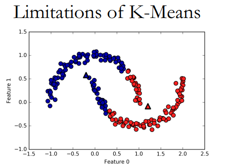
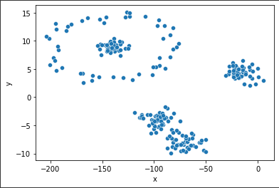
K均值的局限性在于对于这类的数据拟合力较弱:
对于这样的数据集进行Kmeans:
1
2
3
4
5
6
7
import pandas as pddf = pd.read_csv("cluster_data.csv" ) X = df[['x' ]] y = df.y import seaborn as snssns.scatterplot(x="x" , y="y" , data=df)
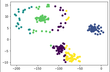
1
2
3
4
5
6
from sklearn.cluster import KMeansmodel = KMeans(n_clusters=5 , random_state=0 ) model.fit(X, y) import matplotlib.pyplot as pltplt.scatter(x = X, y = y, c=model.labels_)
可以看出其局限性。
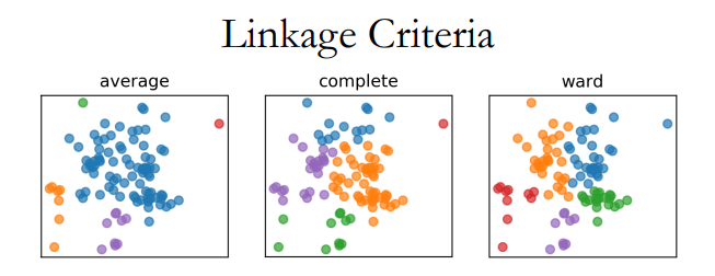
聚合聚类(Agglomerative Clustering) 聚合聚类,或者叫层次聚类(Hierarchical Clustering),与K均值不同,此方法无需预先指定想得到的分类数量。用户在结果中选取即可:
对于这种方法,需要选取不同的连接标准(Merging(Linkage) Criteria)
可以看出这类算法的局限性:连接标准的选取对于模型影响极大。
用法:
1
2
3
4
5
6
from sklearn.cluster import AgglomerativeClusteringfrom sklearn.pipeline import Pipelinefrom sklearn.preprocessing import MinMaxScalerscaler = MinMaxScaler() model = Pipeline([('scaler' , scaler), ('Agglo' , AgglomerativeClustering())]) model.fit(df)
基于密度的噪点空间聚类(Density-Based Spatial Clustering of Applications with Noise) Density-Based Spatial Clustering of Applications with Noise,简称DBSCAN。其核心思想是将密度高的点划分到统一簇中。
需要调节的参数有:
$(\epsilon,MinPt)$
对于前文提到的数据集,采取DBSCAN:
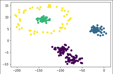
1
2
3
4
5
6
from sklearn.preprocessing import MinMaxScalerscaler = MinMaxScaler() model = Pipeline([('scaler' , scaler), ('DBSCAN' , DBSCAN(eps=0.1 , min_samples=4 ))]) model.fit(df) plt.scatter(x = X, y = y, c=model[1 ].labels_)
可见在参数调整好后,效果还是可以的。
有些时候,我们可以用聚类算法提取特征数据。
1
2
3
4
5
6
7
from sklearn.linear_model import LogisticRegressionfrom sklearn.model_selection import GridSearchCVkm = KMeans(n_init=1 , init="random" ) pipe = make_pipeline(km, LogisticRegression()) param_grid = {'kmeans__n_clusters' : [10 , 50 , 100 , 200 , 500 ]} grid = GridSearchCV(pipe, param_grid, cv=5 , verbose=True ) grid.fit(X, y_people)
聚类模型评估(Clustering Evaluation) 轮廓系数(Silhouette Score) 一个反应聚类结果一致性的标准,可以用于评估聚类后簇与簇之间的离散程度。取值为负一到一,越大越好。
调整兰德指数(Adjusted Rand Index) 简称ARI,也是一个评价指标。数学计算这里略过,本人不搞理论研究,没什么参考必要。
目测法 字面意思,看起来是好的就是好的。
未完待续…
由于当前内容已经超出本文目录结构所能承载的极限,故本文完结,后续内容将在[机器学习基础笔记(三)] 中继续。