机器学习基础笔记(一)
前言
说起当下时兴的知识,我想机器学习绝对是绕不开的一个话题。近些年来,机器学习可以说渗透到了各个领域,到处都贴满了这个概念,仿佛一个项目不说自己使用了机器学习,就落后于了时代。
作为一个目前在读金融分析的学渣,坦白来说,本人是并不太认可在金融领域应用机器学习的,原因很简单:时下的各类机器学习模型,数学层面已经相当复杂,因此很多时候,应用机器学习的人自己都未必知道模型该如何解释,常常是先把模型跑出来再说,至于模型是否有道理、为啥有效、何时无效等则不管不顾。当然了,这不局限于金融行业,很多其他行业也是把机器学习当成黑盒,跑出结果就行,至于过程如何,没人关心。反正先把投资人的钱赚了再说。
然而,本人的意见有些偏激,也不一定合理,自然也微不足道。事实上,机器学习已然在金融行业规模化使用,本人所在实习的公司的部分投组模型也应用了机器学习算法,本学渣也尝试问过老板,在投资上使用黑盒是否合理,不过得到的答复也是说这不是很重要,有结果就行。
无论如何,笔者也还是跟着潮流,选了机器学习的课程。然而作为一个文科生,这玩意对于本人的负载确实有些大了。事实上,对于许多模型底层的数理推导,本人上完课也只是一知半解,实际掌握的更多的只是调库使用。然而即便仅掌握到如此水平,遗忘速度还是惊人的快,因此有必要进行一些笔记整理,增强下理解,以免期末时痛苦万分。
当然,目前课程还未结束,本文会随着课程进度,同步更新。
由于当前内容已经超出本文目录结构所能承载的极限,故本文完结,后续内容将在[机器学习基础笔记(二)]中继续。
概述
什么是机器学习(What is Machine Learning)
这部分内容没什么用,就是纯形而上的定义,但是为了文章的结构完整,我还是将其放在这里:
Large amount of structured and unstructured data
Machine Learning helps capturing the knowledge from the data to improve the performance of predictive models and make data-driven decisions
当然也有各类百科上的定义,如维基:
Machine learning (ML) is the study of computer algorithms that can improve automatically through experience and by the use of data. It is seen as a part of artificial intelligence. Machine learning algorithms build a model based on sample data, known as training data, in order to make predictions or decisions without being explicitly programmed to do so. Machine learning algorithms are used in a wide variety of applications, such as in medicine, email filtering, speech recognition, and computer vision, where it is difficult or unfeasible to develop conventional algorithms to perform the needed tasks.
机器学习的分类(Types of Machine Learning)
这部分内容也没什么用,就是概述性质。
机器学习主要分为下述三类:
- 监督式学习
- 非监督式学习
- 强化学习
都是非核心内容,不多写了,以后有心情再补。
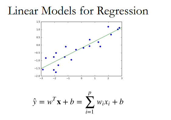
线性回归模型(Linear Regression)
线性回归,可以说是回归模型的核心了,其最简单实现的内容便是拟合出数据的线性函数,如下图:
1 | from sklearn.linear_model import LinearRegression |
最小二乘法(Ordinary Least Squares)
为了计算出上述的拟合线,最小二乘法(OLS)是最重要且最基础的算法。
其核心思想是求预测值减实际值(即残差)的平方和的最小值:

当然,最小二乘法在实际使用中,有很多不足,本人的数学理论水平一般,就不再这深入探讨了,总而言之,由于遇到了模型过拟合问题(Over Fitting),前人对OLS法进行了正则化,这就引出了下文的两种回归。
正则化(Regularization)
正则化一词,一眼看过去就知道不是中文表述了,事实上,这个词的翻译很难做,毕竟中文中没有很好的对应表述,所以,虽然本人认为“正则化”这个翻译很差劲,但我也没什么其他建议,也只好就这么将就用着。
从词义来看,其和“正常化”意思很像,而具体实现的也是把“不正常(过拟合)”的模型变“正常”的过程。
以本学渣的数学水平,是研究不明白正则化的具体算法的,只能记录下其宏观意义所做的事情。简单来说,正则化引入了“惩罚”的概念,具体则是通过一定数学手段,在我们对一个模型引入新的变量时给予”惩罚“。

本人目前学到的正则化主要分为两种:L1正则化以及L2正则化。
对于L1正则化,其将系数权重的绝对值作为惩罚项。
L1正则化可以产生稀疏权值矩阵,即产生一个稀疏模型(有许多系数为零的模型),可以用于特征选择。

而对于L2正则化,其将系数权重绝对值的平方作为惩罚项。
L2正则化可以防止模型过拟合(overfitting),当然一定程度上,L1也可以防止过拟合;它不会使系数变为零,只会使不合适的系数无限靠近零;

多项式化特征(Polynomial Features)
很多时候,我们会拿到形状不是一条直线,而是一条曲线的数据,这时,直接使用线性回归便无法很好拟合曲线,于是,我们想到可以对自变量进行变化,加上指数,这便是多项式变化。
例如对于数据$a,b$,经过二维变换后,便得到$a^2, a, 2ab, b^2, b$三项,此时再进行回归则可得到类二次函数的曲线,而非直线。而同理,我们也可以将多变量进行多维度的变换。
1 | from sklearn.preprocessing import PolynomialFeatures |
数据放缩(Scaling)
这里直接引用比较正式的定义,描述的已经很清晰了:
数据放缩,在统计学中的意思是,通过一定的数学变换方式,将原始数据按照一定的比例进行转换,将数据放到一个小的特定区间内,比如0
1或者-11。目的是消除不同样本之间特性、数量级等特征属性的差异,转化为一个无量纲的相对数值,结果的各个样本特征量数值都处于同一数量级上。
1 | ### 一般与Pipeline共同使用 |
套索回归(LASSO Regression)
LASSO,全称为Least Absolute Shrinkage and Selection Operator,由此其实可知,将其翻译为“套索”是不合理且无意义的。然而,查翻译的时候我发现似乎大家已然习惯这么叫了,那我也就沿用这个名字用下去了。
套索回归本质上就是基础线性模型的L1正则:

1 | ### 一般与Pipeline共同使用 |
岭回归(Ridge Regression)
岭回归本质上就是基础线性模型的L2正则:

1 | ### 一般与Pipeline共同使用 |
弹性网算法(Elastic Net)
弹性网本质上是结合了套索以及岭回归的正则项的算法。

1 | from sklearn.linear_model import ElasticNet |
监督式学习(Supervised Learning)
网格搜索(Grid Search)
在前文介绍的几个模型中,都存在超参数(Hyperpramater),这是在模型开始拟合前,手动输入的一个参数,其直接决定了模型的好坏。
当然,具体超参是什么,它是如何出现的底层原理本人不想深究,总之只要知道调参这一概念即可。
而要进行最优的参数选择,很直觉地,我们便考虑输入多次参数,然后观察模型的表现好坏,选表现最好时的超参作为我们的结果,而这实际上就是穷举法。在编程里很好实现,只要写循环语句即可。这种穷举法被称为网格搜索。
例如我们想用MSE作为模型好坏评估标准,进行网格搜索:
1 | avalues=list(np.logspace(-3, 3, 130)) |
当然,实际使用时我们不去每次都写循环,而是调用GridSearchCV函数:
1 | from sklearn.model_selection import GridSearchCV |
K折交叉验证(K-Fold Cross-Validation)
在以往的例子中,我们都将数据集分为训练集和测试集,然而这样做的问题在于,只随机取了部分样本,这部分是否能代表整体是不好说的,于是,便出现了交叉验证,其将数据多次分割,确保都参与了建模过程。

这K个模型分别在验证集中评估结果,最后的误差MSE加和平均就得到交叉验证误差。我们选取平均误差最低的一项的超参使用。
1 | from sklearn.model_selection import KFold |
最近邻居算法(Nearest Neighbors)
很好理解,简单来说,该算法是用来分类的,未知点的类型判断为与离它最近的点的类型。

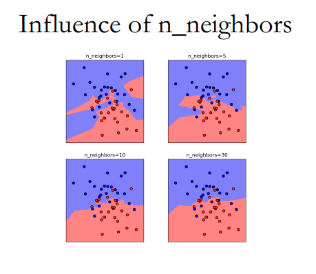
K-近邻算法(K-Nearest Neighbors)
也叫KNN算法,与近邻本质相同,不过将邻居数扩大至K个,然后再“民主投票”决定结果。

邻居数的影响:
利用训练、验证、测试集进行KNN:
1 | X_trainval, X_test, y_trainval, y_test = train_test_split(X, y) |
当然,上述过程也可以使用网格搜索方程实现:
1 | from sklearn.model_selection import GridSearchCV |
数据填补及特征选取(Imputation and Feature Selection)
数据填补(Imputation)
在数据分析中,可以说我们拿到的绝大部分原数据都是存在相当多缺陷的,其中,以数据缺失为代表。
当数据缺失时,不仅会影响到最终的模型结果,有时甚至会让整个数据处理无法进行,因此有必要将缺失数据进行填补,主要方法有:
数据丢弃
这一方式最简单直接,当数据有缺失时,直接丢弃全部的列
1
2
3
4
5
6
7from sklearn.pipeline import make_pipeline
from sklearn.preprocessing import StandardScaler
nan_columns = np.any(np.isnan(X_train), axis=0)
X_drop_columns = X_train[:, ~nan_columns]
logreg = make_pipeline(StandardScaler(), LogisticRegression(solver='lbfgs',multi_class='multinomial'))
scores = cross_val_score(logreg, X_drop_columns, y_train, cv=10)
np.mean(scores)当然,这种方式并不合理,仅仅作为最终手段使用。
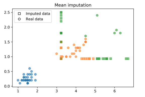
均值/中位数
顾名思义,我们可以利用均值或中位数填补缺失值:
1
2
3from sklearn.preprocessing import Imputer
imp = Imputer(strategy='mean').fit(X_train)
imp.transform(X_train)[-30:]得到的数据分布如:
KNN
K近邻法为:找寻K个最近的非空数据,将其均值赋予空数据
1
2
3
4
5
6
7
8
9
10
11
12
13
14
15distances = np.zeros((X_train.shape[0], X_train.shape[0]))
for i, x1 in enumerate(X_train):
for j, x2 in enumerate(X_train):
dist = (x1 - x2) ** 2
nan_mask = np.isnan(dist)
distances[i, j] = dist[~nan_mask].mean() * X_train.shape[1]
neighbors = np.argsort(distances, axis=1)[:, 1:]
n_neighbors = 3
X_train_knn = X_train.copy()
for feature in range(X_train.shape[1]):
has_missing_value = np.isnan(X_train[:, feature])
for row in np.where(has_missing_value)[0]:
neighbor_features = X_train[neighbors[row], feature]
non_nan_neighbors = neighbor_features[~np.isnan(neighbor_features)]
X_train_knn[row, feature] = non_nan_neighbors[:n_neighbors].mean()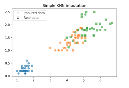
建模法
建模法指利用已有数据建模,来预测缺失数据,如随机森林填补:1
2
3
4
5
6
7
8
9
10
11
12
13
14
15rf = RandomForestRegressor(n_estimators=100)
X_imputed = X_train.copy()
for i in range(10):
last = X_imputed.copy()
for feature in range(X_train.shape[1]):
inds_not_f = np.arange(X_train.shape[1])
inds_not_f = inds_not_f[inds_not_f != feature]
f_missing = np.isnan(X_train[:, feature])
rf.fit(X_imputed[~f_missing][:, inds_not_f], X_train[~f_missing, feature])
X_imputed[f_missing, feature] = rf.predict(
X_imputed[f_missing][:, inds_not_f])
if (np.linalg.norm(last - X_imputed)) < .5:
break
scores = cross_val_score(logreg, X_imputed, y_train, cv=10)
np.mean(scores)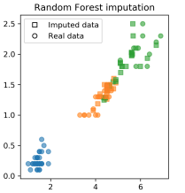
特征选取(Feature Selection)
为什么要进行特征选取,而不是尽可能多的塞特征?
- 优化模型计算速度
- 优化储存空间
- 增加模型解释性
数据降维(Dimensionality Reduction)
主成分分析(Principal Component Analysis)
主成分分析,简称PCA,是一个主要用作数据降维的手段。数学上即为将一组变量通过正交变换转变成另一组线性不相关变量的分析方法,其中这些不相关变量称为主成分(Principal Component)
具体的数学推导对于本人来说难以理解,且即便看懂了,一天后就会忘记,故不在此进行记录,网上资料多的是,这里主要记录作业中的一些代码实现。
1 | # import PCA from sklearn. |
1 | # Transform X_train using PCA. Assign the output to a variable X_train_pca. |
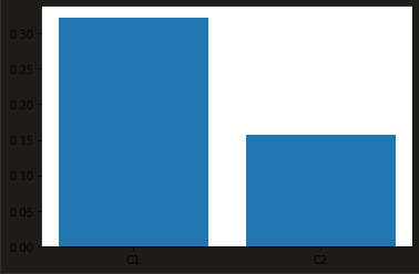
1 | # Plot explained_variance_ratio_ in a bar chart. |
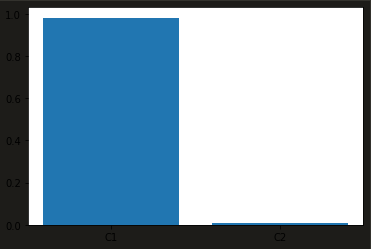
1 | # How do the original features contribute to the first components = pca.components_ |
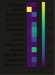
这里我们发现,直接对原数据进行PCA,得到的结果并不好,只有一个主成分显著,且只有一个原特征参与了主成分1的构建。
这种情况是由于我们没有对数据进行无量纲化处理,于是引入数据放缩库:
1 | from sklearn.pipeline import make_pipeline |
可见数据放缩后,各主成分都起到了解释方差的作用。
绘制不同的主成分数对于整体数据的解释力:
1 | pca_scaled = make_pipeline(StandardScaler(), PCA(n_components=12)) |
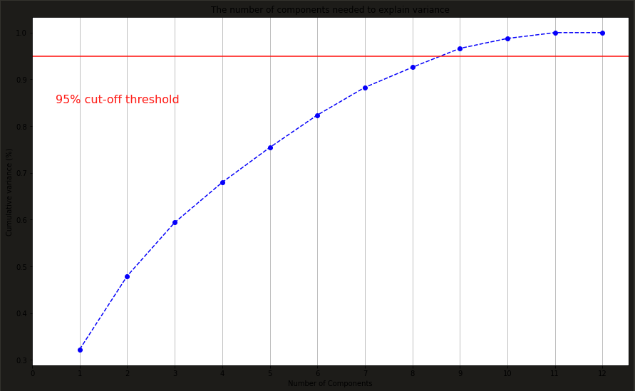
可以看出,当主成分为8时,即可解释原数据的95%的方差,这时我们便实现了将原有的12维数据降至8维。
预处理及特征工程(Preprocessing and Feature Engineering)
预处理
这里主要介绍了不同的数据放缩方法,前文有涉及,故在此不多赘述。
分类特征处理(Categorical Feature)
对于机器学习建模,我们最常见的当然是数字类型的特征(Numerical Data),然而,直觉地,我们也会想去考虑类别这一影响因素,如性别、地名等,而这一类的特征原数据并非数字,因此无法直接纳入模型中,分类特征处理便是为了解决如何将这些特征数字化,使其可以被模型计算。
丢弃分类特征(Drop Categorical Feature)
顾名思义,这一方法说的是当我们遇到分类特征时,直接丢弃。实则是当鸵鸟逃避问题,没什么用,这里不再赘述。
序号编码(Ordinal Encoding)
这一方法说的是将分类特征转换为0~N-1的数。
假设我们有以下数据:
1 | import pandas as pd |
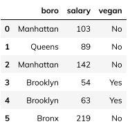
我们对boro一列进行序号编码:
1 | df['boro_ordinal'] = df.boro.astype("category").cat.codes |
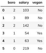
这里可以看出,序号编码虽然给每个分类都赋了值,然而其数字意义不明,对于模型的可读及可解释性负面影响很大,于是便有了接下来的独热编码。
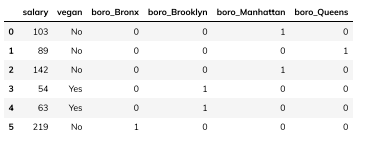
独热编码(One-Hot Encoding)
独热编码相较序号编码,增加了N列,每列代表原列的一个分类,用1和0表示是否属于这个类别:
1 | pd.get_dummies(df.columns=['boro']) |
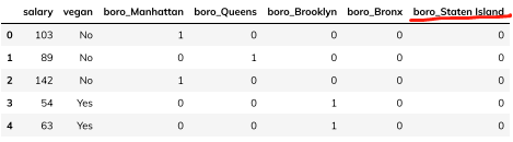
当然,也可以自定义想要的类名,如果原数据本身没有这一类:
1 | df = pd.DataFrame({ |
对于独热编码来说,虽然其容易实现,然而问题也是很明显的:
首先,其增加了新的特征列,尤其是用人名等分类多的特征做独热处理时,很容易使我们的数据维度变得极大,这对机器学习十分不利。
另外,独热编码会使数据集出现非常多的0,让机器学习模型难以处理。
同时,其数据存在冗余资讯、多重共线性等等问题,并不是一个很好的处理手段。
频率编码(Frequency Encoding)
频率编码指将某个分类出现的频率数量作为其数值。
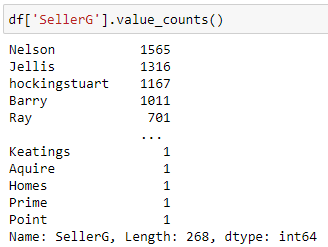
这种方式的问题在于,如果有类别出现频数一致,那么模型会误认为其为同一个类别。
目标编码(Target Encoding)
目标编码指把同样类别的数据对应的「目标值」全部拿到,并且将这些值做平均,用作新编码的值。
效果:
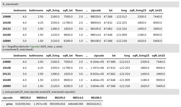
使用:
1 | pip install category_encoders |
当然,这种方式也有不足,如利用了目标值来做编码,某种程度上可以理解为用目标值的一部分来预测目标值,而这会引发过拟合问题;同时,在使用这种方式时,还要注意处理异常值,因为异常值会对均值有较大影响。
列转换(Column Transformer)
我们可以将上述编码方式装入列转换方法,然后封装到pipeline中:
1 | categorical = df.dtypes == object |
如果我们想对于类别特征以及数字特征分别进行编码和放缩,则可以使用pipeline嵌套在ColumnTransformer中的方式:
1 | model = Pipeline(steps=[('preprocessor', |
未完待续…
由于当前内容已经超出本文目录结构所能承载的极限,故本文完结,后续内容将在 [机器学习基础笔记(二)] 中继续。